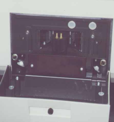
The principles of molecular fluorescence are covered in your text.
In brief, a high-energy photon (the excitation frequency) is absorbed and
it raises the molecule to an excited state. As the excited molecule relaxes
to a lower excited level or to the ground state, the excess energy is released
to the molecular environment by a variety of mechanisms. One of these relaxation
processes is fluorescence. With fluorescence, light is emitted (the
emission frequency) at the same or at a lower frequency than the excitation
frequency. See Fraiji, Hayes and Werner, J. Chem. Ed., vol. 69, page
424, 1992 for a simple and relatively complete discussion of the different
relaxation reactions and their rates). The other relaxation mechanisms
are frequently more efficient than fluorescence so only a few molecules
fluoresce. However, for those molecules that do fluoresce, one usually
obtains very low detection limits. Progress is being made in
attaching fluorescence tags to molecules that do not fluoresce.
The quantum yield (Q), sometimes called the quantum efficiency, is the ratio of the molecules that fluoresce to those that are excited. Q = If / (Io – I) where If is the intensity (power) of the fluorescence beam Io is the intensity (power) of the excitation beam and I is the intensity of the beam after it is some distance into the sample. Therefore, If = Q(Io-I) And from the Beer law, A = log Io/I = eC l or 10A = Io/I or I=Io /10A = Io10–A so that If = Q(Io-Io10–A) and If = QIo(1-10–A) which is the working equation for fluorescence spectroscopy. Note that the equation is not linear so you should not expect
a plot of fluorescence versus concentration to be
a straight line. However, at very low concentrations (when A is less
than 0.05), the equation approaches a straight line and at even lower concentrations
the degree of curvature is negligible.
|
In this experiment, you will determine the exact amount of quinine
in various liquids (tonic water and colas). The approximate concentration
is 100 ppm. You will then determine the extent of the quenching by sodium
chloride, the type of quenching (static, dynamic or both) and the second
order rate constant for the quenching process assuming the fluorescence
lifetime for quinine without any quencher is 19.02 nano-seconds (Phillips,
J. Photochem., vol. 23, page 193, 1983) and the fluorescence quantum yield
at infinite dilution and at 25 Co for quinine is 0.546 (Melhuish,
J. Phys. Chem., vol. 65. p. 229, 1961).
The applicable form of the Stern-Volmer equation that you will use to determine the quenching rate constant is Io / I = 1 + K [Cl-] where Io is the intensity without quencher, I is the intensity with quencher . It is apparent from this equation that a graph of the ratio of the fluorescence intensity without salt to that with salt plotted against the concentration of salt will give a straight line with a slope of K. The quantum yield is related to the intensity of a fluorescence peak by the factor (1-10–A) where A is the absorbance of quinine at the excitation wavelength. If you assume the factor is small, you can estimate the rate constant from the ratios of the fluorescence peak heights as follows. Taking into account the lifetime of fluorescence , the quenching constant K can be written as K = Kq x t , where Kq is the 2nd order quenching rate constant and t is the fluorescence lifetime of quinine (19.02 ns) : K = Kq x 19.02 x 10⁻⁹ s You might want to measure the absorbance of the quinine solution you use for the quenching study at the excitation wavelength and correct the fluorescence peak height data. A diffusion controlled rate constant pertains to a chemical reaction
in which the reactants react as quickly as they are able to diffuse through
the solvent and come in contact with one another. If the quenching
rate constant is the same as the diffusion-controlled rate constant, one
interpretation would be that every collision between an excited quinine
molecule and a chloride ion results in a transfer of energy from the quinine
(so it does not fluoresce) to the chloride.
Preparation of solutions:
|
Instrument Operation:
Turn the instrument on and wait 15 min. Open the FLWinLab program (just click on icon). Load quinine method. For 10-7 M solution, run Pre-scan prcedure. Fix maximum of emission and run exitation spectrum from 230 to 390 nm. Fix maximum of excitation and run emission spectrum from 400 to 500 nm. Repeat the same procedure with other peaks at excitation spectra. Compare excitation spectrum to the absorption spectrum of quinine. Procedure for Quinine Determination: By trial and error, dilute your stock solution to get a linear calibration curve (fluorescence intensity versus concentration). Start in the vicinity of 10-7 M and use the linear part of your curve to estimate detection limit of method and sensetivity. Include both the calibration curve and the spectra in your report. Analyze your sample using teh calibration. Process results. Analyze your sample once again using standard addition method You may also want compare your results with UV/vis data. Quenching. After you have finished analyzing your unknown, measure the fluorescence of five solutions of quinine with concentrations in the high, but linear, part of your calibration curve and with 0.003, 0.005, 0.010, 0.020 and 0.0400 moles/l of sodium chloride added to the sulfuric acid-quinine solutions. Plot the ratio of the intensities (fluorescence peak heights) without and with the sodium chloride as a quencher against the salt concentration. You should get a straight line. Include the graph (with slope, intercept and correlation coefficient) in your report. Determine the type of quenching process you have, calculate the rate constant for the quenching process using the Stern-Volmer equation and the fluorescence lifetime of quinine given above and compare your results with the diffusion limited second order rate constant (k) (Fraiji, Hayes and Werner, J. Chem. Ed., vol. 69, page 424, 1992 ). The viscosity of the sodium chloride solution (assume water) at 20C is approximately 0.010 Poise. Explain any difference between the rate constant you obtain using fluorescence data and the diffusion-limited rate constant you calculate using viscosity data. |
Report:
1. Excitation and emission spectra of quinine.
2. Calibration curve for quinine determination. Be sure your calibration curve shows the origin and the upper limit of the linear region of the curve. Include a rigorous determination of the reliability of your data and an estimate of the lowest detection limit for quinine you can obtain using this general fluorescence method and after optimizing all instrument variables to enable you to measure the lowest possible concentration of quinine. 3. Detection limit and determination limit for quinine. 4. Your estimate of quinine concentration in your sample using both calibration and standard addition procedures. 5. Quenching of quinine flurescence with NaCl. Include all constants you have aclculated. Also include an evaluation of your results relative to the theories of fluorescence spectroscopy and of the quenching mechanisms. Include a discussion of what you learned by comparing the relaxation rate constant you determined from fluorescence data with that calculated for a diffusion-limited process. |